A guide to running the model
Here we provide an overview of the suggested method for running the model. The model used here closely corresponds to that of Lee (1997). There are two files in the example_runs directory that provide a starting point for running the model. The suggested method is to first spin up the model using the L97_WC4_init.jl file. Then the user runs the L97_WC4_SS.jl file to initialize the model from the end of the spin-up run, and compute steady-state statistics of the turbulent flow. We now provide more details on these files. First, we provide some background on the model setup.
Basic picture
The model in these examples damps the perturbation flow to a background state that i) has constant zonal flow in a meridional band in the center of the domain, and ii) tapers to zero at the boundaries. The parameter WC sets the half-width of the baroclinic zone. As WC gets wider, the background state transitions from having one to multiple jets. A main focus of Lee (1997) is characterizing these jet-state transitions.
Paths
The example scripts define a few paths, required to run the model: - src_dir: This is the directory to the source code. Please change accordingly - save_path: This is where data from the model runs will be saved.
I suggest making separate directories for the init runs and the SS runs (and for each WC value).
fig_path: This is where automatically generated figures will be saved.
restart_path: This is used in the SS file to tell the code where to look for the initial conditions. This should be the save_path from the init file.
Saving data
There are two ways to save data. The first is by setting save_bool = true. This will save snapshots of the upper and lower-layer streamfunctions at periods specified via the save_every variable. In addition, this only saves a band of data centered in the middle of the domain, to save memory (since there generally isn’t much happening near the walls). The meridional width of this band is specified via the y_width parameter, where 1 will save the whole channel and 0.5, for example, will only save the middle half of the channel.
The second option for saving data is by setting save_last=true. This will save a complete snapshot of the upper and lower streamfunction at the end of the model run, so that the snapshot can be used for initial conditions for future runs.
Plotting
Two plotting functions are currently defined in the output_fcns.jl file. These plots can be saved every plot_every time steps by setting either plot_basic_bool or plot_BCI_bool to true, respectively.
To add your own plot - Create a plotting function in the output_fcns.jl file, analogous
to the pre-existing ones
Add a conditional statement in the run_model() function (in init_fcns.jl), analogous to the two current plot options
Set the plot-related boolean that you used in the conditional statement equal to true in your model run file
Model initialization and spin-up
Open the L97_WC4_init.jl file. Define the appropriate paths for finding source code, saving data, and possibly saving figures.
Steady-state model run
After running L97_WC4_init.jl, you should have a restart file saved. Now open L97_WC4_SS.jl. Define the four appropriate paths (src_dir, save_path, fig_path, and restart_path).
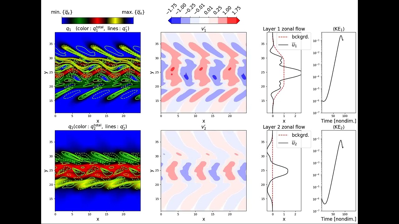
We suggest setting the plot_basic_bool boolean to true, in order to see some interesting time-dependent behavior of the flow.
Next steps
Some possible next steps are - Change the WC parameter (i.e., the width of the baroclinic zone)
and see how this affects both i) unstable mode growth, and ii) turbulence
Create different plotting functions to visualize different time-dependent behaviors of the flow (e.g., compute time-dependent zonally-averaged PV gradient)
Output snapshots of data with enough frequency to compute, for example, energy budgets in wavenumber-space, wavenumber-integrated energy budgets, frequency-wavenumber spectra, or time-averaged momentum budgets